17  EM: the Expectation-Maximization Algorithm

library(here)
library(knitr)
library(mixtools)
library(tidyverse)

# resolve conflicts with plotly
# conflicted::conflicts_prefer(plotly::layout)

# resolve conflicts with tidymodels packages
# tidymodels::tidymodels_prefer()

library(eda4mlr)

# stabilize simulated data
source(here("code", "eda4ml_set_seed.R"))

---

17.1 Background

Latent Dirichlet Allocation (LDA) was proposed as a method of topic modeling in 2003 in a paper by Blei, Ng, and Jordan. The method is briefly mentioned in Part 1 of the course. Several course participants requested a more detailed description. This note prepares for the requested response by introducing the EM Algorithm.¹

17.2 Example: Old Faithful eruptions

17.2.1 Delay and Duration

The figure below represents the duration of eruptions (“duration”) and the interval between eruptions (“delay”)² of the “Old Faithful” geyser in Yellowstone National Park, Wyoming from August 1 to August 15, 1985.³

faithful_tbl <- datasets::faithful |> 
  tibble::as_tibble() |> 
  dplyr::rename(
    duration = eruptions, 
    delay    = waiting
  ) |> 
  dplyr::select(delay, duration)

g_faithful_tbl <- faithful_tbl |> 
  ggplot2::ggplot(mapping = ggplot2::aes(
    x = delay, y = duration
  )) + 
  ggplot2::geom_point() + 
  ggplot2::labs(title = "Old Faithful eruptions: delay and duration") + 
  ggplot2::xlab("delay (minutes") + 
  ggplot2::ylab("duration (minutes")
g_faithful_tbl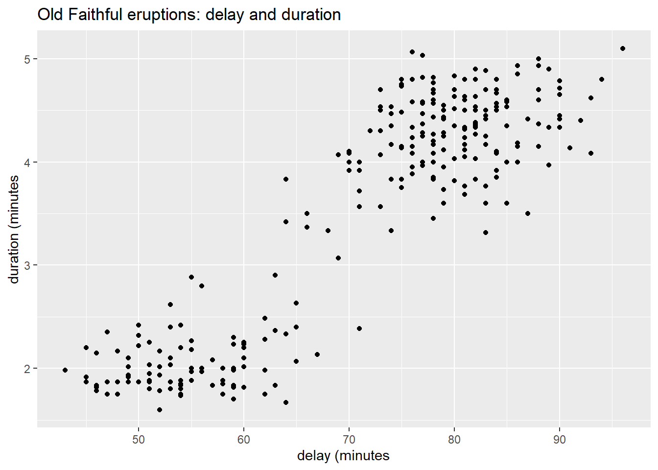

Figure 17.1: Old Faithful eruptions: delay and duration (minutes)

17.2.2 Gausian Mixture Model

The figure shows two clusters of data points.⁴ Here is probability model in which the delay and duration of each eruption follows one of two possible bivariate normal distributions depending on the group, \(G\), to which it belongs.

\[ \begin{align} \{ \; (\text{delay}, \text{duration}) \; | \; \text{group } G \; \} &\sim \mathcal{N}(\mu_{\bullet}^{(G)}, \Sigma^{(G)}) \\ \\ & \text{where } \\ \\ G &= \begin{cases} 1 & \text{with probability } p_1 \\ 2 & \text{with probability } p_2 = 1 - p_1 \end{cases} \end{align} \qquad(17.1)\]

Averaging across the two groups, a randomly selected eruption has the following mixture of bivariate normal distributions.

\[ \begin{align} (\text{delay}, \text{duration}) &\sim p_1 \; \mathcal{N}(\mu_{\bullet}^{(1)}, \Sigma^{(1)}) + p_2 \; \mathcal{N}(\mu_{\bullet}^{(2)}, \Sigma^{(2)}) \\ \\ & \text{where } p_1 + p_2 = 1\\ \end{align} \qquad(17.2)\]

Fitting a single multivariate normal distribution is straightforward⁵, but less so for the above mixture of bivariate normal distributions. The Expectation-Maximization (EM) algorithm provides an approach for doing so, as follows.

17.2.3 Latent Variable: Cluster Membership

In the EM framework, we iteratively assign group-membership, \(G = g \in \{ 1, 2 \}\), to each data point. Based on this set of assignments we update the parameter estimates (the “E” step of the EM algorithm). The new set of parameter estimates yields a new estimate of the likelihood function. We then re-assign cluster-membership to maximize the updated likelihood estimate (the “M” step). The iteration terminates once the magnitude of changes falls below a prescribed threshold.

In R this procedure is implemented by the function mixtools::mvnormalmixEM().

17.2.4 Initial Estimates

Based on the preceding figure we adopt the following initial estimates of the parameters.

1. Calculate the respective medians of the (delay, duration) variables.

2. For each data point determine whether the delay value is less than the median of all observed delay values. Similarly determine whether the duration value is less than the median of all observed duration values.

3. Based on these inequalities, categorize each (delay, duration) data point as belonging to one of four groups: (lower, lower), (lower, upper), (upper, lower), (upper, upper).

4. Restrict attention to the (lower, lower), and (upper, upper) groups. Within this restricted set of data points calculate the sample averages and covariance matrices for each of the two groups. Use these as initial estimates of \((\mu_{\bullet}^{(1)}, \mu_{\bullet}^{(2)})\) and \((\Sigma^{(1)}, \Sigma^{(2)})\).

The table below summarizes the groups delineated by the respective medians of (delay, duration).

faithful_4 <- faithful_tbl |> 
  dplyr::mutate(
    delay_low     = delay    < median(delay), 
    duration_low  = duration < median(duration)
  )

faithful_4_smy <- faithful_4 |> 
  dplyr::summarise(
    .by           = c(delay_low, duration_low), 
    count         = n(), 
    delay_mean    = mean(delay), 
    duration_mean = mean(duration), 
    delay_sd      = sd(delay), 
    duration_sd   = sd(duration), 
    dd_cor        = cor(delay, duration), 
    delay_var     = var(delay), 
    duration_var  = var(duration), 
    dd_cov        = cov(delay, duration)
  )

faithful_4_smy |> 
  dplyr::select(delay_low, duration_low, count:dd_cor) |> 
  knitr::kable(
    caption = "Summary statistics for initial groups of data points", 
    digits = 1
  )

Table 17.1: Summary statistics for initial groups of data points

Summary statistics for initial groups of data points

delay_low	duration_low	count	delay_mean	duration_mean	delay_sd	duration_sd	dd_cor
FALSE	TRUE	22	81.1	3.7	3.5	0.2	-0.2
TRUE	TRUE	112	56.6	2.2	7.7	0.6	0.7
FALSE	FALSE	116	82.4	4.5	4.6	0.3	0.1
TRUE	FALSE	22	73.0	4.4	1.9	0.3	0.6

Restricting attention to the groups in which (delay, duration) jointly fall either below or above their respective medians, we extract the initial parameter estimates from the table above. Variable g is the labeling of each point in the restricted data set to cluster 1 or cluster 2.

faithful_2 <- faithful_4 |> 
  dplyr::filter(delay_low == duration_low) |> 
  dplyr::mutate(
    g = dplyr::if_else(delay_low, 1L, 2L)
  ) |> 
  dplyr::select(g, delay, duration)

initial_est <- faithful_4_smy |> 
  dplyr::filter(delay_low == duration_low) |> 
  dplyr::mutate(
    g      = dplyr::if_else(delay_low, 1L, 2L), 
    ct_sum = sum(count), 
    p      = count/ct_sum
  ) |> 
  dplyr::select(
    g, count, p, delay_mean:dd_cov
  )

initial_est |> 
  dplyr::select(g, count, delay_mean:dd_cor) |> 
  knitr::kable(
    caption = "Initial parameter estimates", 
    digits = 1
  )

Table 17.2: Initial parameter estimates

Initial parameter estimates

g	count	delay_mean	duration_mean	delay_sd	duration_sd	dd_cor
1	112	56.6	2.2	7.7	0.6	0.7
2	116	82.4	4.5	4.6	0.3	0.1

The figure below summarizes results so far. We’ve restricted attention to data points (delay, duration) such that the two variables are either both below their respective medians or else both above their respective medians. We’ve defined variable g as the grouping variable taking integer values (1, 2) in these two respective cases. For each of the two groups we’ve constructed an ellipse conforming to the sample mean vector and covariance matrix of the group. The ellipse is designed to capture 50% of the area under a bivariate normal distribution having these parameter values.

delay_median    <- faithful_tbl$delay    |> median()
duration_median <- faithful_tbl$duration |> median()

g_faithful_2 <- faithful_2 |> 
  dplyr::mutate(g = forcats::as_factor(g)) |> 
  dplyr::group_by(g) |> 
  ggplot2::ggplot(mapping = ggplot2::aes(
    x = delay, y = duration, colour = g
  )) + 
  ggplot2::geom_point(
    mapping = ggplot2::aes(colour = g, shape = g), 
    show.legend = TRUE
  ) + 
  ggplot2::geom_vline(xintercept = delay_median) + 
  ggplot2::geom_hline(yintercept = duration_median) + 
  ggplot2::stat_ellipse(level = 0.5) + 
  ggplot2::labs(
    title = "Old Faithful eruptions: initial normal estimates", 
    subtitle = "50% normal ellipses for quadrants 1 and 3"
  )
g_faithful_2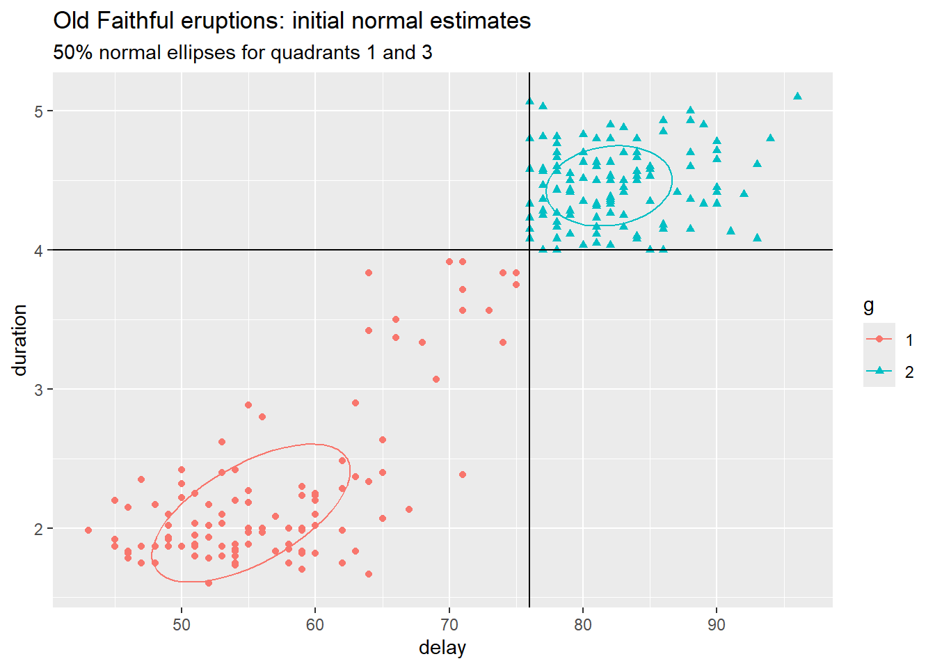

Figure 17.2: Old Faithful eruptions: initial normal estimates

This completes the initial “E” step in the EM algorithm, the estimation of parameter values.

17.2.5 Log Likelihood

We now begin the initial “M” step (maximization) of the EM algorithm. Using the above parameter estimates we now assign cluster membership (variable g) to the points not yet labeled by maximizing the likelihood function, or equivalently (and more conveniently), the logarithm of the likelihood function.

In general, recall that a multivariate normal distribution having mean vector \(\mu_{\bullet} \in \mathbb{R}^m\) and covariance matrix \(\Sigma\) has likelihood function equal to the product of the multivariate normal density evaluated at each observation vector, say \(x_{\bullet}^{(\nu)}\), (that is, at each row of the design matrix \(X\)).

\[ \begin{align} \mathcal{L}(X, \mu_{\bullet}, \Sigma) &= \prod_{\nu = 1}^n \mathcal{N}(x_{\bullet}^{(\nu)} - \mu_{\bullet}, \; \Sigma) \end{align} \]

Taking the natural logarithm of both sides of this equation, we obtain the log-likelihood function.

\[ \begin{align} \mathcal{l}(X, \mu_{\bullet}, \Sigma) &= \sum_{\nu = 1}^n \log_e(\mathcal{N}(x_{\bullet}^{(\nu)} - \mu_{\bullet}, \; \Sigma)) \\ &= -\frac{m}{2} \log_e(2 \pi) - \frac{1}{2}\log_e(\det{\Sigma}) - \frac{1}{2} \sum_{\nu = 1}^n (x_{\bullet}^{(\nu)} - \mu_{\bullet})^{\intercal} \; \Sigma^{-1} (x_{\bullet}^{(\nu)} - \mu_{\bullet}) \\ \end{align} \]

Consequently, fitting parameters \(\mu_{\bullet}\) and \(\Sigma\) to the design matrix \(X\) via maximum likelihood amounts to minimizing the sum of quadratic forms on the right side of this equation. (Each term in the sum is referred to as the squared Mahalanobis distance between the observation vector and the mean vector.)

\[ \begin{align} (\hat{\mu}_{\bullet}, \hat{\Sigma}) & = \arg \min \sum_{\nu = 1}^n (x_{\bullet}^{(\nu)} - \mu_{\bullet})^{\intercal} \; \Sigma^{-1} (x_{\bullet}^{(\nu)} - \mu_{\bullet}) \\ \end{align} \]

which yields the sample mean and a variant of the sample covariance matrix.

\[ \begin{align} \hat{\mu}_{\bullet} & = \frac{1}{n} \sum_{\nu = 1}^n x_{\bullet}^{(\nu)} \\ \\ \hat{\Sigma} & = \frac{1}{n} \sum_{\nu = 1}^n (x_{\bullet}^{(\nu)} - \hat{\mu}_{\bullet}) (x_{\bullet}^{(\nu)} - \hat{\mu}_{\bullet})^{\intercal} \\ \end{align} \]

For the Old Faithful data, however, we propose a mixture of two distnct normal distributions, that is, two clusters in which the cluster to which each data point belongs is unknown.

Having estimated the normal parameters for clusters 1 and 2, we now label each data point as belonging to the cluster to which it is closest, in the sense of Mahalanobis distance. The results are shown in the next figure.

f_mu <- c(initial_est$delay_mean, initial_est$duration_mean) |> 
  matrix(nrow = 2, ncol = 2)
colnames(f_mu) <- c("delay", "duration")

f_sigma <- list()

f_sigma[[1]] <- c(
  initial_est$delay_var    [[1]], 
  initial_est$dd_cov       [[1]], 
  initial_est$dd_cov       [[1]], 
  initial_est$duration_var [[1]]
) |> 
  matrix(nrow = 2, ncol = 2)

colnames(f_sigma [[1]]) <- c("delay", "duration")
rownames(f_sigma [[1]]) <- c("delay", "duration")

f_sigma[[2]] <- c(
  initial_est$delay_var    [[2]], 
  initial_est$dd_cov       [[2]], 
  initial_est$dd_cov       [[2]], 
  initial_est$duration_var [[2]]
) |> 
  matrix(nrow = 2, ncol = 2)

colnames(f_sigma [[2]]) <- c("delay", "duration")
rownames(f_sigma [[2]]) <- c("delay", "duration")

f_tag_tbl <- faithful_tbl |> 
  dplyr::rowwise() |> 
  dplyr::mutate(
    md_1 = mahalanobis(
      x      = c(delay, duration), 
      center = f_mu    [1, ], 
      cov    = f_sigma [[1]]
    ), 
    md_2 = mahalanobis(
      x      = c(delay, duration), 
      center = f_mu    [2, ], 
      cov    = f_sigma [[2]]
    ), 
    g = dplyr::if_else(md_1 < md_2, 1L, 2L)
  )
f_tag_tbl <- f_tag_tbl |> 
  dplyr::ungroup()

g_f_tag_tbl <- f_tag_tbl |> 
  dplyr::mutate(g = forcats::as_factor(g)) |> 
  dplyr::group_by(g) |> 
  ggplot2::ggplot(mapping = ggplot2::aes(
    x = delay, y = duration, group = g
  )) + 
  ggplot2::geom_point(
    ggplot2::aes(
      colour = g, 
      shape  = g, 
    ), 
    show.legend = TRUE
  ) + 
  ggplot2::geom_vline(xintercept = delay_median) + 
  ggplot2::geom_hline(yintercept = duration_median) + 
  ggplot2::labs(
    title = "Old Faithful: inital clustering of all points", 
    subtitle = "with original quadrants defined by medians"
  )
g_f_tag_tbl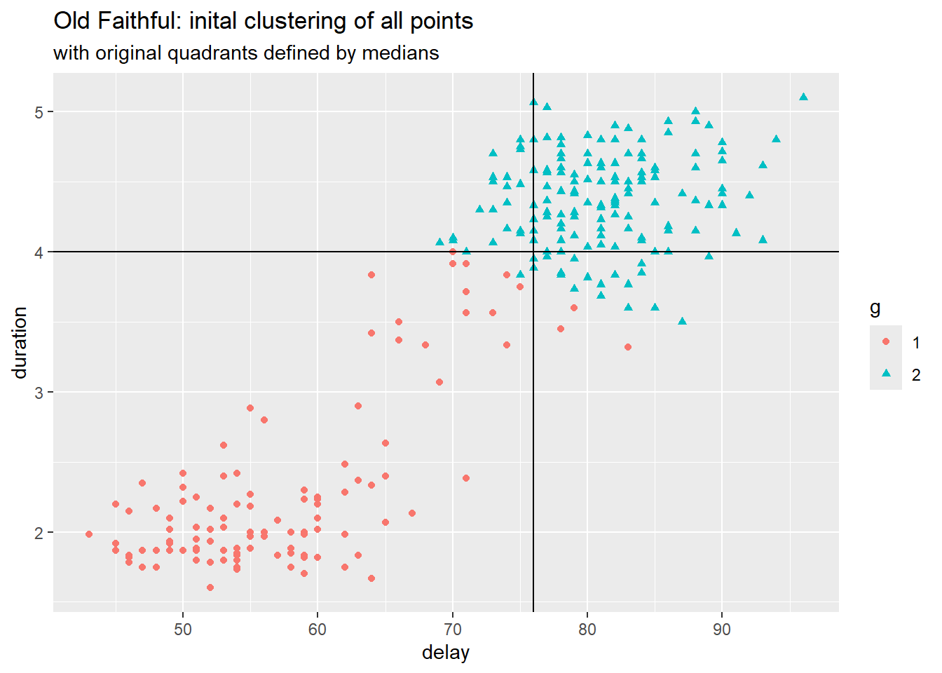

Figure 17.3: Old Faithful: inital clustering of all points

This completes the initial maximization step. The table below shows the revised summary statistics per cluster now that the initial assignment to clusters has been completed.

f_tag_smy <- f_tag_tbl |> 
  dplyr::ungroup() |> 
  dplyr::summarise(
    .by = g, 
    count         = n(), 
    delay_mean    = mean(delay), 
    duration_mean = mean(duration), 
    delay_sd      = sd(delay), 
    duration_sd   = sd(duration), 
    dd_cor        = cor(delay, duration), 
    delay_var     = var(delay), 
    duration_var  = var(duration), 
    dd_cov        = cov(delay, duration)
  )

f_tag_smy |> 
  dplyr::select(g:dd_cor) |> 
  knitr::kable(
    caption = "Summary statistics for initial clusters of data points", 
    digits = 1
  )

Table 17.3: Summary statistics for initial clusters of data points

Summary statistics for initial clusters of data points

g	count	delay_mean	duration_mean	delay_sd	duration_sd	dd_cor
1	115	57.1	2.3	8.4	0.6	0.7
2	157	81.0	4.4	5.3	0.3	0.1

17.3 EM Iterations

We illustrate the iterations of the EM algorithm using function mvnormalmixEM() in R package mixtools.⁶ We provide the function with our initial estimates of normal parameters.

em_out <- faithful_tbl |> 
  mixtools::mvnormalmixEM(
    lambda = c(0.5, 0.5), 
    mu = list(
      # delay, duration
      c(56.6, 2.25), # (lower, lower)
      c(82.4, 4.47)  # (upper, upper)
    ), 
    sigma = list(
      # (lower, lower)
      matrix(
        nrow = 2, ncol = 2, 
        data = c(
          59.7,  3.27, 
          3.27,  0.35
        )), 
      # (upper, upper)
      matrix(
        nrow = 2, ncol = 2, 
        data = c(
          21.5,  0.19, 
          0.19,  0.08
        ))
    ), 
    verb = TRUE
  )

iteration= 1 diff= 41.60226 log-likelihood -1168.518 
iteration= 2 diff= 14.54077 log-likelihood -1153.978 
iteration= 3 diff= 12.21481 log-likelihood -1141.763 
iteration= 4 diff= 9.461094 log-likelihood -1132.302 
iteration= 5 diff= 1.962679 log-likelihood -1130.339 
iteration= 6 diff= 0.0717014 log-likelihood -1130.267 
iteration= 7 diff= 0.003089365 log-likelihood -1130.264 
iteration= 8 diff= 0.000168951 log-likelihood -1130.264 
iteration= 9 diff= 9.661982e-06 log-likelihood -1130.264 
iteration= 10 diff= 5.582749e-07 log-likelihood -1130.264 
iteration= 11 diff= 3.233686e-08 log-likelihood -1130.264 
iteration= 12 diff= 1.874241e-09 log-likelihood -1130.264 
number of iterations= 12 

Reports from each iteration were requested by setting function parameter verb = TRUE (verbose). The estimated log-likelihood is shown for each iteration, along with the change in that value from the previous iteration.

The final estimates of the normal parameters are shown in the table below, and illustrated in the figure below.

f_em <- faithful_tbl |> 
  dplyr::bind_cols(em_out$posterior) |> 
  dplyr::mutate(
    g = dplyr::if_else(comp.1 > comp.2, 1L, 2L)
  )

f_em_smy <- f_em |> 
  dplyr::summarise(
    .by           = g, 
    count         = n(), 
    delay_mean    = mean(delay), 
    duration_mean = mean(duration), 
    delay_sd      = sd(delay), 
    duration_sd   = sd(duration), 
    dd_cor        = cor(delay, duration), 
    delay_var     = var(delay), 
    duration_var  = var(duration), 
    dd_cov        = cov(delay, duration)
  ) |> 
  dplyr::arrange(g)

f_em_smy |> 
  dplyr::select(g, count:dd_cor) |> 
  knitr::kable(
    caption = "Summary statistics for final groups of data points", 
    digits = 1
  )

Table 17.4: Summary statistics for final groups of data points

Summary statistics for final groups of data points

g	count	delay_mean	duration_mean	delay_sd	duration_sd	dd_cor
1	97	54.5	2.0	5.8	0.3	0.3
2	175	80.0	4.3	6.0	0.4	0.4

g_f_em <- f_em |> 
  dplyr::mutate(g = forcats::as_factor(g)) |> 
  dplyr::group_by(g) |> 
  ggplot2::ggplot(mapping = ggplot2::aes(
    x = delay, y = duration, colour = g
  )) + 
  ggplot2::geom_point(
    mapping = ggplot2::aes(colour = g, shape = g), 
    show.legend = TRUE
  ) + 
  ggplot2::geom_vline(xintercept = delay_median) + 
  ggplot2::geom_hline(yintercept = duration_median) + 
  ggplot2::stat_ellipse(level = 0.5) + 
  ggplot2::labs(
    title = "Old Faithful eruptions: final normal estimates", 
    subtitle = "50% normal ellipses for clusters 1 and 2"
  )
g_f_em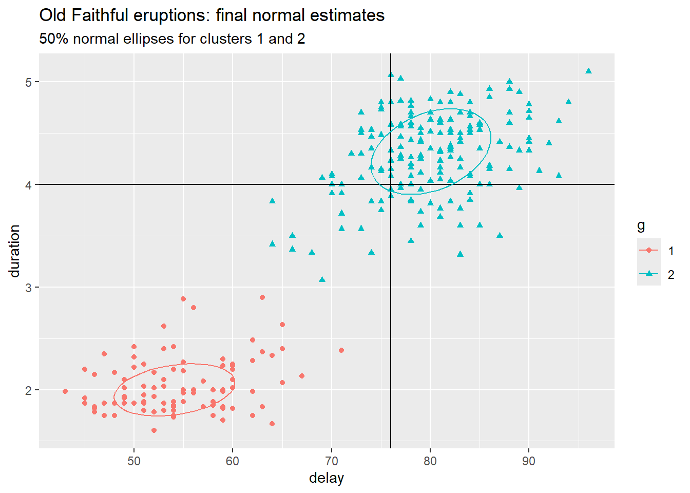

Figure 17.4: Old Faithful eruptions: final normal estimates

17.4 Group Membership over Time

According to the EM algorithm, here is the pattern of group membership as a function of time. More precisely, here is the posterior probability of group-1 membership as a function of cumulative delay expressed in days.

g_grp_per_cum_delay <- f_em |> 
  # cumulative delay in days
  dplyr::mutate(
    cum_delay = cumsum(delay) / (60 * 24), 
    g = forcats::as_factor(g)
  ) |> 
  ggplot2::ggplot(mapping = ggplot2::aes(
    x = cum_delay, y = comp.1, color = g, fill = g)) + 
  ggplot2::geom_point(
    mapping = ggplot2::aes(colour = g, shape = g), 
    show.legend = TRUE) + 
  ggplot2::labs(
    title = "Group 1 posterior probability over cumulative delay (days)") + 
  ggplot2::xlab("cumulative delay (days)") + 
  ggplot2::ylab("group 1 posterior probability")
g_grp_per_cum_delay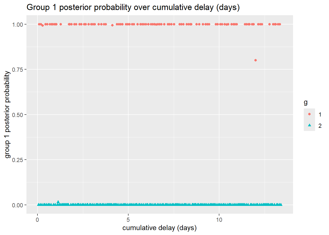

Figure 17.5: Group 1 posterior probability over cumulative delay (days)

Recall that group 1 refers to the eruptions having shorter delays and shorter durations. The figure shows that these are interupted by short stretches of eruptions from group 2. The figure also show that posterior probabilities come out to be nearly zero or else nearly unity, with rare exceptions.

17.5 Closing Remarks

Several papers present the mathematics underlying the EM algorithm, and one can also find tutorials that illustrate the convergence of the algorithm.

17.6 Resources

In addition to the references listed below, see the following.

The EM Algorithm Explained blog by Chloe Bi, 2019

17.7 References

Anderson, T. W., and Ingram Olkin. 2002. “Maximum-Likelihood Estimation of the Parameters of a Multivariate Normal Distribution.” Linear Algebra and Its Applications, May. https://www.sciencedirect.com/science/article/pii/0024379585900497.

Peng, Roger D. 2025. Advanced Statistical Computing. https://bookdown.org/rdpeng/advstatcomp/.

---

1. See Peng (2025, chp. 4), and (EM_algo_Wikipedia_2025?).

2. “Delay” here refers to the length of time preceding the current eruption. The (delay, duration) variables are recorded in minutes.

3. There are two prominent R packages representing the Old Faithful measurements during August, 1985. The MASS::geyser data set of 299 observations includes nocturnal measurements whose duration was coded as 2, 3 or 4 minutes, having originally been described as ‘short’, ‘medium’ or ‘long’. The datasets::faithful data set of 272 measurements, shown in the figure, excludes 27 of these nocturnal measurements.

4. Old Faithful eruptions are conjectured to occur in 2 distinct temporal patterns due to the presence of an upper and lower chamber beneath the vertical column (tube) that forms the geyser. See (Vandemeulebrouck_Roux_Cros_2013?).

5. See Anderson and Olkin (2002).

6. See (mixtools2009?).